On this page
quick_reference_all
Plotting
How to plot the result graph or the Pareto front
Plotting Results
Visualization is a powerful way to interpret and present the results of your community detection analysis. Here, we show how to:
- Plot the community-labeled graph from a solution
- Plot the Pareto front to understand trade-offs
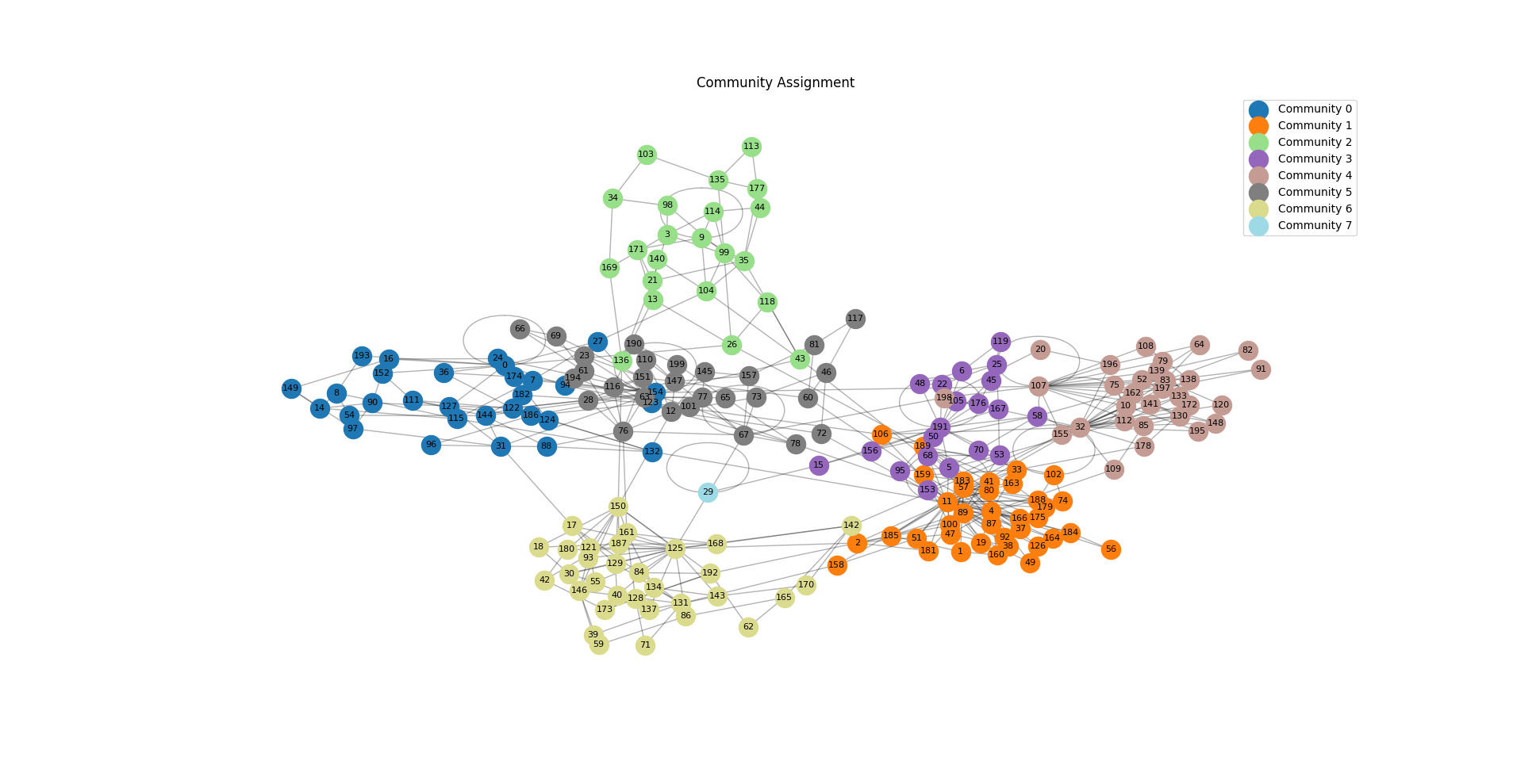
Plotting the Community Graph
After obtaining a solution (either from .run() or from generate_pareto_front()), you can visualize the graph with nodes colored by their assigned communities.
  import matplotlib.pyplot as plt
import networkx as nx
import matplotlib.cm as cm
import numpy as np

def plot_communities(G, labels):
    pos = nx.spring_layout(G, seed=42)
    communities = list(set(labels.values()))
    color_map = cm.get_cmap('tab20', len(communities))

    for idx, c in enumerate(communities):
        nodes = [n for n in G.nodes if labels[n] == c]
        nx.draw_networkx_nodes(
            G,
            pos,
            nodelist=nodes,
            node_color=[color_map(idx)],
            label=f'Community {c}'
        )

    nx.draw_networkx_edges(G, pos, alpha=0.3)
    nx.draw_networkx_labels(G, pos, font_size=8)
    plt.title("Community Assignment")
    plt.legend()
    plt.axis('off')
    plt.show()
Example Usage:
  import networkx as nx
import pymocd

G = nx.LFR_benchmark_graph(200, 3, 1.5, 0.1, average_degree=5, min_community=20, seed=2)
alg = pymocd.HpMocd(graph=G)

solution = alg.run()
plot_communities(G, solution)
Or, from the Pareto front:
  frontier = alg.generate_pareto_front()
labels, _ = frontier[23]
plot_communities(G, labels)
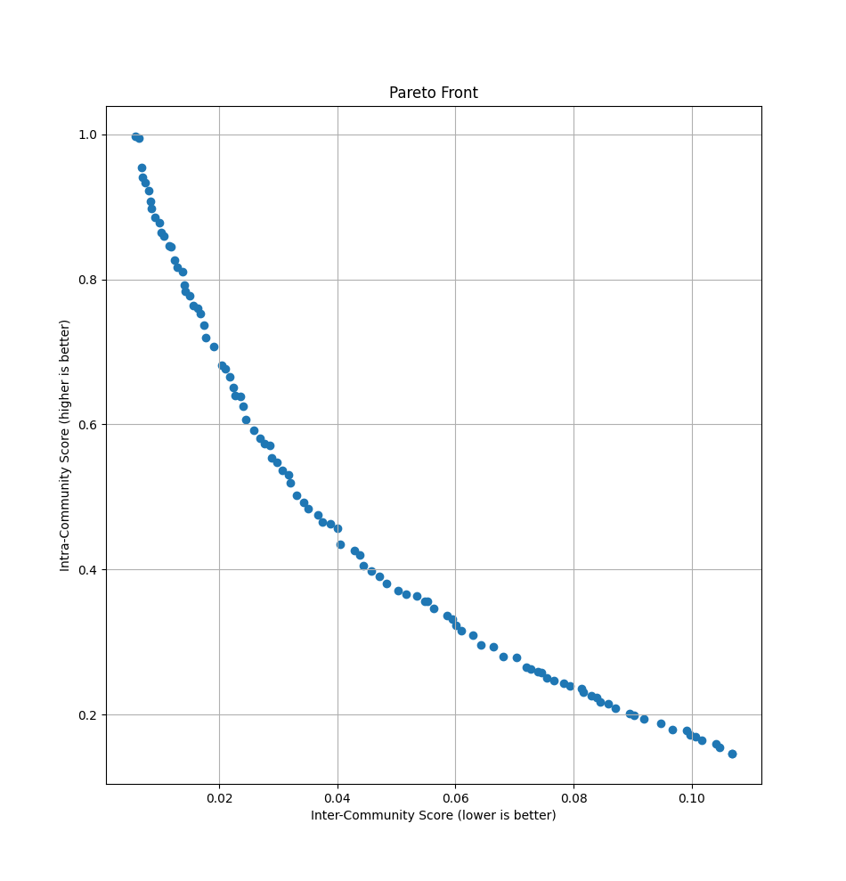
Plotting the Pareto Front
To visualize the trade-offs between intra- and inter-community metrics across solutions, plot the Pareto front itself.
  def plot_pareto_front(frontier):
    intra = [entry[1][0] for entry in frontier]
    inter = [entry[1][1] for entry in frontier]

    plt.figure()
    plt.scatter(inter, intra, marker='o')
    plt.xlabel("Inter-Community Score (lower is better)")
    plt.ylabel("Intra-Community Score (higher is better)")
    plt.title("Pareto Front")
    plt.grid(True)
    plt.show()
Example Usage:
plot_pareto_front(frontier)
Expected Outputs
Last updated 02 Jun 2025, 18:19 -0300 .